pymultipact package
Submodules
pymultipact.domain module
-
class pymultipact.domain.Domain(project, boundary_file=
None, field=None, n_boundary_points=250, **kwargs)[source]¶ Bases:
object-
analyse_multipacting(mode=
1, xrange=None, epks=None, phis=None, v_init=2, integrator='rk4', step=None, proc_count=None, loss_model='field')[source]¶ Analyse multipacting. The Epk sweep is run in parallel by default.
- Parameters:
- mode : int
Eigenmode index
- xrange : list, ndarray
Range of surface emission sites (z interval)
- epks : list, ndarray
Peak surface electric field sweep values [V/m]
- phis : list, ndarray
Initial phases
- v_init : float, int
Particle emission energy [eV]
- integrator : str
Numerical integration scheme
- step : float
Minimum distance between emission sites
- proc_count : int or None
Number of worker processes for the Epk sweep. None (default) chooses automatically from the machine’s CPU count and the number of sweep points; 1 runs in-process without spawning workers. Note for Windows scripts: guard the call with
if __name__ == '__main__':(multiprocessing spawn requirement); notebooks are fine as-is.- loss_model : str
What happens to an electron impacting the wall while the surface field is unfavourable (E.n < 0): ‘field’ absorbs it (paper behaviour, default); ‘wait’ re-emits it uncounted until the RF phase turns favourable (MultiPac-style delayed re-emission); ‘always’ re-emits and counts the impact (upper bound).
-
analyse_multipacting_parallel(proc_count=
1, mode=1, xrange=None, epks=None, phis=None, v_init=2, integrator='rk4', step=None)[source]¶ Deprecated alias – analyse_multipacting is parallel by default now.
- calculate_Ef()[source]
Mean FINAL impact energy of the electrons that reached 20 hits (the bright set) – zero wherever nothing survived to 20 hits, exactly like the paper’s Ef_20. Computing this over the leftover particles instead produced spurious out-of-band spikes from runaway lost particles.
- calculate_distance_function(particles, lmbda)[source]
Distance function d_20 of each bright (20-hit) trajectory, Yla-Oijala Eq. (3.2.3): the distance in (position, phase) space between the initial point (emission site, launch phase) and the 20th impact point. Minima locate the fixed points of resonant multipacting orbits. Stored in particles.df20, aligned with bright_set.
- compute_fields()[source]
Solve the eigenmodes.
- Parameters:
- order : int
Finite element order. 3 (default) matches MultiPac’s third-order elements and keeps field accuracy on the coarser resampled boundary/mesh; the original code used order=1 on a very dense surface mesh.
-
define_elliptical_cavity(mid_cell=
None, lend_cell=None, rend_cell=None, beampipe='None')[source]¶ - Parameters:
- mid_cell : list, ndarray
Array of cavity middle cells’ geometric parameters
- lend_cell : list, ndarray
Array of cavity left end cell’s geometric parameters
- rend_cell : list, ndarray
Array of cavity left end cell’s geometric parameters
- beampipe : str {"left", "right", "both", "none"}
Specify if beam pipe is on one or both ends or at no end at all
-
launchable_fraction(mode=
1)[source]¶ Fraction of the launched (site, phase) combinations whose surface field at emission allows the electron to leave the wall (E.n >= 0). For a sinusoidal field this is ~0.5: half of all initial phases die on their first impacts. MultiPac’s counter function effectively counts only launchable electrons in c0, so to compare against MultiPac divide cn_c0 by this fraction (see plot_cf(launchable_norm=True)).
-
plot_cf(launchable_norm=
False)[source]¶ Counter function. launchable_norm=True divides by the fraction of launchable initial electrons (E.n >= 0 at emission, ~0.5), which is the normalisation MultiPac’s c20/c0 effectively uses.
-
plot_df(epk_i, metric=
'd20', vmax=None)[source]¶ MultiPac-style distance map over (emission site, initial phase) for the epk_i-th field level of the sweep. Grey cells = no electron survived to 20 impacts from that (site, phase).
- Parameters:
- epk_i : int
Index into the Epk sweep (self.epks_v).
- metric : str
‘d20’ (default): distance between the initial (site, phase) and the nearest of the last two impacts. For two-point multipacting the orbit returns to the launch side only on every other impact, so taking the closer of impacts 19 and 20 removes the arbitrary branch parity: launches at the resonant phase give d ~ 0 (dark core) and off-core launches grow with their phase offset – the same graded structure as MultiPac’s d20 map. ‘d20_strict’: the literal Yla-Oijala Eq. 3.2.3 (20th impact only). Carries a ~pi phase offset whenever the 20th impact lands on the opposite branch. ‘closure’: distance between the 20th and 18th impacts (closure of the two-impact map); zero for any phase-locked orbit.
- vmax : float, None or 'kappa'
Colour scale maximum. ‘kappa’ (default for ‘d20’) clips at lambda/(2 pi) like MultiPac’s d20 display; None autoscales.
- set_sey(sey_filepath)[source]
Set custom secondary emission yield
-
track_particles(mode=
1, integrator='rk4')[source]
-
analyse_multipacting(mode=
- class pymultipact.domain.Project[source]
Bases:
object- create_project(folder_path)[source]
- load_project(folder_path)[source]
- class pymultipact.domain.SEY(sey_filepath)[source]
Bases:
object
pymultipact.geometry_writer module
- pymultipact.geometry_writer.f(z, *data)[source]
Calculates the coordinates of the tangent line that connects two ellipses
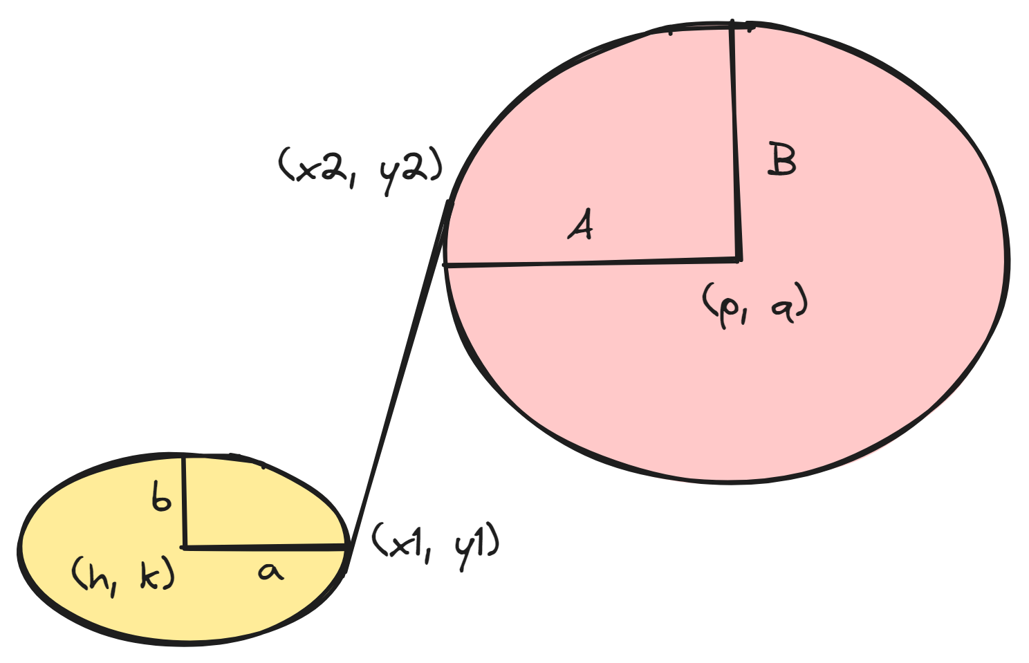
Note
The four returned non-linear functions are
\[ \begin{align}\begin{aligned}f_1 = \frac{A^2b^2(x_1 - h)(y_2-q)}{a^2B^2(x_2-p)(y_1-k)} - 1\\f_2 = \frac{(x_1 - h)^2}{a^2} + \frac{(y_1-k)^2}{b^2} - 1\\f_3 = \frac{(x_2 - p)^2}{A^2} + \frac{(y_2-q)^2}{B^2} - 1\\f_4 = \frac{-b^2(x_1-x_2)(x_1-h)}{a^2(y_1-y_2)(y_1-k)} - 1\end{aligned}\end{align} \]
- pymultipact.geometry_writer.jac(z, *data)[source]
Computes the Jacobian of the non-linear system of ellipse tangent equations
-
pymultipact.geometry_writer.linspace(start, stop, step=
1.0)[source]¶ Like np.linspace but uses step instead of num This is inclusive to stop, so if start=1, stop=3, step=0.5 Output is: array([1., 1.5, 2., 2.5, 3.])
-
pymultipact.geometry_writer.write_ell_cavity(folder=
None, mid_cell=None, lend_cell=None, rend_cell=None, beampipe=None, name=None, step=None, n_cell=None, plot=False)[source]¶ Write cavity geometry to be used for multipacting analysis
- Parameters:
- folder : str
Folder path to write geometry to
- n_cell : int
Number of cavity cells
- mid_cell : list, ndarray
Array of cavity middle cells’ geometric parameters
- lend_cell : list, ndarray
Array of cavity left end cell’s geometric parameters
- rend_cell : list, ndarray
Array of cavity left end cell’s geometric parameters
- beampipe : str {"left", "right", "both", "none"}
Specify if beam pipe is on one or both ends or at no end at all
- plot : bool
If True, the cavity geometry is plotted for viewing
-
pymultipact.geometry_writer.write_ell_cavity_flat_top(folder=
None, mid_cell=None, lend_cell=None, rend_cell=None, name=None, step=None, n_cell=None)[source]
pymultipact.integrators module
-
class pymultipact.integrators.Integrators(mesh, w, bounding_rect, loss_model=
'field')[source]¶ Bases:
object- collision(active_interval)[source]
- compose_indices(indices_array)[source]
- update_lpi(lpi, removed_inds)[source]
- update_rpi(rpi, removed_inds)[source]
pymultipact.field_interpolator module
Field access objects for PyMultipact.
Two implementations share one interface so they are interchangeable in the integrator:
.e(points)        -> (N, 2) complex   bulk E field; RAISES if any point is
                                      outside the domain (this drives the
                                      exception-based boundary detection)
.h(points)        -> (N, 1) complex   bulk H field (same raise behaviour)
.e_exact(point)   -> (1, 2) complex   exact FEM E at a single point
.h_exact(point)   -> (1, 1) complex   exact FEM H at a single point
.is_inside(points)-> (N,)  bool       true-polygon inside test
EMFieldDirect evaluates the FEM solution directly everywhere (accurate, matches the paper; slow because ngsolve must locate every point in the unstructured mesh).
FastFieldCache precomputes E/H on a regular grid once and does O(1) bilinear lookups for the bulk force. The field query itself is ~13x faster than exact FEM. HOWEVER it is NOT viable for multipacting and is kept only for reference: the surviving electrons live in a sub-millimetre layer at the wall and bounce ~20 times, so they need (a) a boundary criterion that matches the mesh exactly – the polygon is slightly larger than the meshed region, so a grid raise lets particles penetrate the wall and be lost (wrong counter function), and (b) near-exact near-wall fields – small grid errors compound over the bounces and throw the impact energies off by several fold. Using an exact mesh-based raise fixes the counter function but removes the speed-up (mesh point-location is back) and the energies are still wrong. In short: a global grid cannot cheaply resolve the near-surface physics; accurate fields here require ngsolve’s mesh point-location (which is the real cost, and why a compiled code like Multipac is faster – it is largely a language, not an algorithm, gap for the field query).
-
class pymultipact.field_interpolator.EMFieldDirect(gfu_E, gfu_H, mesh, boundary, bounding_rect=
None, resolution=None)[source]¶ Bases:
objectDirect FEM point evaluation (accurate, slow). Interface as above.
-
class pymultipact.field_interpolator.FastFieldCache(gfu_E, gfu_H, mesh, boundary, bounding_rect, resolution=
500)[source]¶ Bases:
objectStructured-grid field lookup for the bulk force + exact FEM at impacts.
pymultipact.main module
pymultipact.multipac_plot module
- pymultipact.multipac_plot.get_files_from_directories(root_folder, keyword)[source]
- pymultipact.multipac_plot.get_power_from_directories(root_folder, keyword)[source]
-
pymultipact.multipac_plot.plot_cst_pic_results(folders, label, Eaccs_eigen, Eacc, xlim=
None, ylim=None)[source]
-
pymultipact.multipac_plot.plot_electron_evolution_spark3d(filename, power_folder, Eacc, sep=
'\\s+', layout=None)[source]
-
pymultipact.multipac_plot.plot_multipac_triplot(Eacc_list, Epk_Eacc_list, folders, labels, kind=
'triplot', layout=None, min_max=None, hist=None)[source]
-
pymultipact.multipac_plot.plot_trajectory(files_folder, loc=
'center')[source]
pymultipact.multipact module
pymultipact.particles module
-
class pymultipact.particles.Particles(xrange, init_v, bounds, phi, cmap=
'jet', step=None)[source]¶ Bases:
object