Multipacting analysis of the TESLA mid-cell
This example reproduces the benchmark of the PyMultipact paper (IPAC’24, MOPS27): the mid-cell of the TESLA cavity is meshed, its fundamental (TM$_{010}$) mode is solved with NGSolve, and electrons emitted from the equator region are tracked over a sweep of peak surface electric field levels to locate the multipacting band.
See the Theory page for the governing equations and the definitions of the metrics plotted below.
%matplotlib inline
import numpy as np

from pymultipact.domain import Project, Domain
Domain and eigenmode
A Project names the working folder; the Domain reads the TESLA mid-cell
contour, resamples the boundary polyline (~250 points) and meshes it.
compute_fields() solves the Maxwell eigenvalue problem with third-order
Nédélec elements — the TM$_{010}$ frequency of the mid-cell is 1300 MHz.
proj = Project()
proj.create_project('TESLA')

domain = Domain(proj)
domain.compute_fields()
Boundary polyline resampled: 1049 -> 147 points (n_boundary_points=None keeps the full resolution)
Boundary polyline resampled: 1831 -> 147 points (n_boundary_points=None keeps the full resolution)
0 -2.5135035950784276e-14 freq:  nan MHz
1 742.4614307569854 freq:  1300.1030691666238 MHz
2 2656.757500289286 freq:  2459.329913290589 MHz
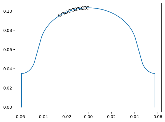
Emission sites
Electrons are launched from surface sites in a window on the equator side of the cell (circles below), each over a full turn of initial RF phases.
xrange = [-0.025, 0.0]
domain.show_initial_points(xrange, step=0.002)
Field-level sweep
analyse_multipacting tracks every (site, phase) electron for 10 RF periods
at each peak-field value. The sweep is parallelised over the field levels by
default (proc_count=None uses the machine’s cores; from a plain script on
Windows, call it under if __name__ == '__main__':).
epks = np.linspace(1, 90, 179) * 1e6          # peak surface field [V/m]
phis = np.linspace(0, 2 * np.pi, 72)          # initial phases

domain.analyse_multipacting(mode=1, epks=epks, phis=phis,
                            xrange=xrange, step=0.002, proc_count=12)
Running Epk sweep (179 points) on 12 processes.
Total runtime::  354.7451310157776
Done with multipacting analysis.
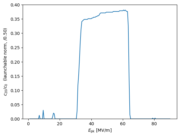
Counter function
The fraction of electrons surviving 20 impacts. The TESLA mid-cell shows its
well-known two-point multipacting band at roughly 29–59 MV/m plus narrow
low-field resonances. launchable_norm=True divides by the ~50% of initial
phases that can actually emit (the normalisation MultiPac uses), making the
curve directly comparable with MultiPac results.
domain.plot_cf(launchable_norm=True)
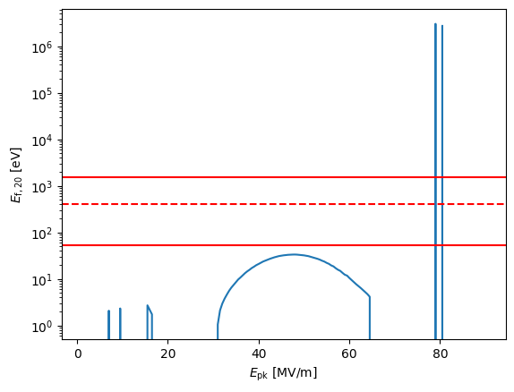
Final impact energy
The mean final (20th) impact energy of the surviving electrons. The solid red lines are the SEY crossover energies ($\delta = 1$) and the dashed line the peak-SEY energy of the surface data: multipacting sustained at impact energies between the crossovers can multiply.
domain.plot_Ef()
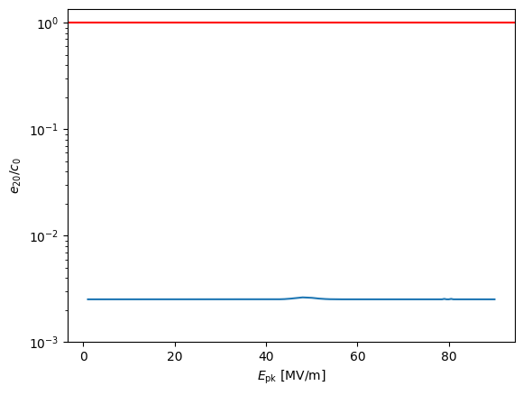
Enhanced counter function
Weights every surviving trajectory by the product of its per-impact secondary yields — values above 1 (red line) mean the electron population truly grows.
domain.plot_ef()
Distance map
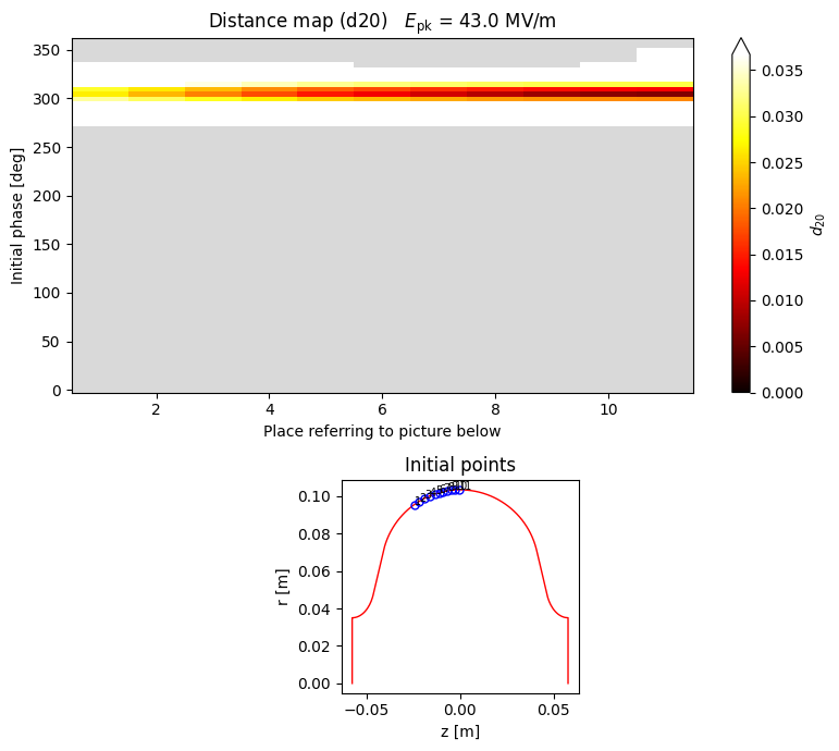
For one field level inside the band, the distance function $d_{20}$
over (emission site, initial phase): the distance between the launch
point and the nearest of the last two impacts (two-point orbits
return to the launch side on every other impact). The dark core marks
the resonant fixed-point phase; the colour grades with the launch
offset from it, and grey cells did not survive to 20 impacts – the
same structure as MultiPac’s $d_{20}$ map. Also available:
metric='d20_strict' (literal thesis definition from the 20th
impact) and metric='closure' (orbit-closure test, 20th vs 18th
impact).
i_band = int(np.argmin(np.abs(epks - 43e6)))   # ~43 MV/m
domain.plot_df(i_band)
Further exploration
domain.plot_trajectories()opens an interactive browser (sliders) over the surviving trajectories of each field level.domain.analyse_multipacting(loss_model=...)switches the treatment of impacts at unfavourable field phase ('field','wait','always').domain.set_sey(path)loads a different secondary emission yield table.Domain(proj, n_boundary_points=None)keeps the full boundary resolution (the original TESLA contour is preserved insample_domains/tesla_mid_cell_fine.n).